Breast Ultrasound Lesion Analysis
Abstract
Two independent models estimate malignancy and delineate the index lesion in breast ultrasound images. Development uses BUS-BRA, with patient-disjoint training, validation and testing partitions. Input resolution and segmentation encoder are selected on validation; the selected configurations are trained with three seeds. Evaluation includes case-level classification, native-resolution segmentation, calibration and error analysis. Saved outputs can be inspected in the image explorer.
1. Data and task definition
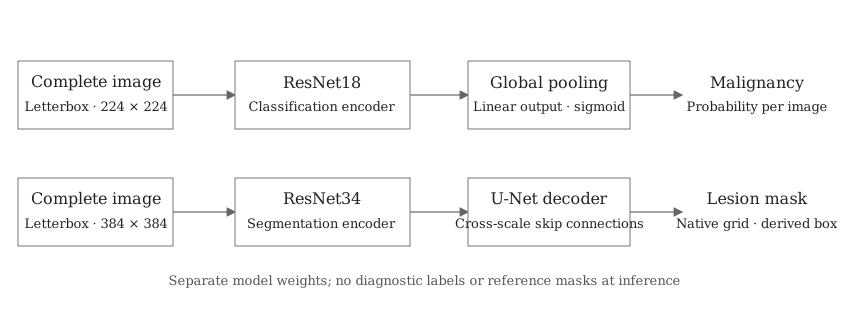
The classifier distinguishes benign from malignant index lesions. The segmenter predicts the annotated index lesion; its largest connected component provides a bounding box. Both models receive the complete image. Expert masks, clinical variables, BI-RADS and filenames are excluded from the model input.
BUS-BRA contains 1,875 images from 1,064 patient cases, with diagnoses and expert masks [1]. All views from one case remain in one partition. The split is stratified by diagnosis, with seed 2026 and intended fractions of 70%, 15% and 15%. Pixel checksums and perceptual hashes are audited before splitting. The released validation columns contain patient overlap with training, so a custom patient split is used.
| Partition | Cases | Images | Benign | Malignant |
|---|---|---|---|---|
| Training | 744 | 1,307 | 505 | 239 |
| Validation | 160 | 286 | 109 | 51 |
| Testing | 160 | 282 | 108 | 52 |
BrEaST contributes a second cohort of 252 lesion images and four normal images [2]. Its results describe transfer to another collection; it is excluded from model and threshold selection. Other-lesion annotations are retained for inspection, without inheriting the index lesion's diagnosis. The available images represent selected lesions, rather than complete examinations or a screening population.
2. Image preparation and models
Images are converted to grayscale, repeated across three channels and normalized using ImageNet statistics. Resizing preserves aspect ratio and pads to a square. Candidate inputs are 224 × 224 and 384 × 384 pixels. Segmentation losses exclude padding; predicted probabilities are restored to the original image grid before scoring.
Classification uses an ImageNet-initialized ResNet18 [3], global average pooling and a linear binary output. Segmentation uses a ResNet18 or ResNet34 encoder and a U-Net-style decoder [4] with skip connections. The decoder channels are 128, 64, 32, 16 and 16. The networks have separate weights and are trained independently.
The selected classifier uses ResNet18 at 224 pixels. The selected segmenter uses U-Net with ResNet34 at 384 pixels. Both configurations are selected using validation only.
| Model | Construction | Output |
|---|---|---|
| Classification | Fine-tuned ResNet18; 224 or 384 px | Single-image malignancy probability; mean across images for a case |
| Segmentation | ResNet18 U-Net at 224 or 384 px; ResNet34 U-Net at 384 px | Index-lesion mask and largest-component box |
| Frozen features | ImageNet ResNet18 at 224 px, weighted standardization and logistic regression | Malignancy probability |
| Controls | Case prevalence and mean spatial mask, calculated on training only | Constant probability and fixed spatial prediction |
The frozen classifier selects regularization from C = 0.01, 0.1, 1 and 10 using validation AP. Controls establish whether image-dependent predictions improve upon prevalence and a fixed lesion position.
3. Training and model selection
Five candidate configurations are fitted with seed 17. Classification checkpoints and configuration are selected by validation average precision (AP) per case; segmentation uses validation Dice per case at native resolution. The two selected configurations are also fitted with seeds 29 and 43, giving nine neural fits in total. Scores used for selection are development estimates.
AdamW uses initial learning rates of 10−4 for the encoder and 10−3 for the output layers, with weight decay 10−4 and cosine decay over 50 epochs. Early stopping has patience 10. Batch size is 16 at 224 pixels and eight at 384 pixels. Mixed precision is used for training; validation and evaluation use float32.
Classification minimizes binary cross-entropy. Segmentation minimizes 0.5 binary cross-entropy + 0.5 Dice loss. Each image is weighted by the inverse number of images in its case. Training augmentation applies horizontal reflection, rotation up to 7°, translation up to 4%, scaling from 0.9 to 1.1, and brightness/contrast changes of up to 10%. Image and mask geometry are transformed together. No annotation-derived crop is used.
4. Evaluation and image inspection
Classification reports AP, AUROC, sensitivity, specificity, precision, F1, balanced accuracy, MCC and Brier score. Probabilities are averaged within each case. The decision threshold maximizes validation Youden J; temperature scaling is a secondary calibration analysis. Both are then fixed for testing. Results at threshold 0.5 are retained.
Segmentation reports case-averaged Dice and IoU, their median and tenth percentile, and derived box overlap. Masks use a fixed threshold of 0.5 at native resolution. Uncertainty is estimated with 2,000 case bootstrap samples; variation across training seeds is reported separately. Device, lesion size and diagnosis strata support error analysis.
The explorer displays saved images with prediction contours, filled masks, boxes and optional reference annotations. Classification and segmentation runs can be selected independently, so their outputs are visible for the same image. All controls affect display only. Quantities can be traced to saved predictions, validation policies and checksums.
Numerical estimates, failed cases and their interpretation are reported in the results article.
5. Reproduction
The implementation uses Python 3.12, PyTorch and TorchVision. Package versions, data checksums, splits, run configurations, training histories and checkpoints are recorded. The executed environment uses an NVIDIA RTX 3070 Laptop with 8 GB of memory.
References
- Gómez-Flores W, Gregorio-Calas MJ, Pereira WCA. BUS-BRA: A breast ultrasound dataset for assessing computer-aided diagnosis systems. Medical Physics, 2024. doi:10.1002/mp.16812.
- Pawłowska A et al. Curated benchmark dataset for ultrasound based breast lesion analysis. Scientific Data, 2024. doi:10.1038/s41597-024-02984-z.
- He K et al. Deep residual learning for image recognition. CVPR, 2016. Paper.
- Ronneberger O, Fischer P, Brox T. U-Net: Convolutional networks for biomedical image segmentation. MICCAI, 2015. Paper.
- Tejani AS et al. Checklist for Artificial Intelligence in Medical Imaging (CLAIM): 2024 update. Radiology: Artificial Intelligence. doi:10.1148/ryai.240300.